Inferential Statistics

When it comes to pursuing a career in Data Science, knowledge of statistics is a must. Without a basic understanding of statistics, it is difficult to master the art of prediction using Data Science and predictive analytics. Whenever we try to find patterns and make predictions based on the data, statistics is always involved. Inferential Statistics utilizes a sample from a large population and makes predictions about a large population from which the sample was observed. To sum up, Inferential Statistics is used to make the estimates for a large population and test the hypothesis to draw the final verdict.

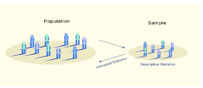
Image Credit: Voxco

 

Example:

Exit polls after every election. For opinion or Exit polls, the news channels take a representative sample from a large population, utilize inferential statistics and make predictions about the election result in the form of an Exit poll.

There are 2 ways by which the prediction can be done here:

1. Channels can collect opinions from every voter of that particular geography and present the Exit poll results
2. Channels can take representative samples of that geographical population and do the prediction about the large population using inferential statistics.

Now, collecting opinions from every voter will take a lot of time, resources, money, and, physical labor. On the other hand, using a representative sample of a large population can solve this problem. Inferential Statistics can be used to make inferences about a large population from the representative sample.

 

Basics of Inferential Statistics

Before going deep into Statistics learners need to have a fundamental understanding of Normal Distribution. In this article, we will focus only on the basics of inferential statistics by understanding the fundamentals of normal distribution.

The normal distribution, also known as the Gaussian distribution, is a symmetric probability distribution concentrated on the mean, indicating that data around the mean occur more frequently than data far from it. On a graph, the normal distribution will appear as a bell curve.

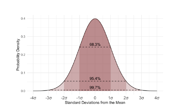
Image credit: Wikimedia Commons

• The area under this curve is always represented as 1. It is a curve where half of the values lie on the left and half of the values lie on the right.
• 3% data falls inside 1 standard deviation (σ) of the population mean (μ)
• 4% data falls inside 2 standard deviations (σ) of the population mean (μ)
• 7% data falls inside 3 standard deviations (σ) of the population mean (μ)x

To calculate the probability of occurrence of an event we need to calculate the z score here. The z score is essentially the standard deviation distance between the value and the mean. A positive z value of 1.2816 indicates that the value is 1.2816 standard deviations away from the mean. The probability is then calculated by looking up the relevant z value in the z table.

The formula to calculate the z-score is

Where,

μ = population mean,

σ = standard deviation,

x = value against which the z-score will be calculated.

Once the z score is calculated, the probability of occurrence of any event can be looked up by referring to the z score from the z table.

The concept of normal distribution derives from the central limit theorem which states that when you take a representative sample from a large population the mean of both the pools is more or less equal. Also, the standard deviation of the sample is equal to the standard deviation of population divided by the square root of sample size.

(σ) Sample = (σ) population / √N

The formula itself says that if you have a large sample size N then the chances of getting a lower standard deviation is high, hence you will get better accuracy in determining the sample mean.

Note: One key ask of the central limit theorem is to have a sample size >30

 

It’s always a question of how well the sampling distribution estimates the actual population. This problem is addressed by a confidence interval. A confidence interval (CI) is a range of values that are expected to include a population figure with a high degree of certainty. A population mean is often expressed as a percentage when it falls between two intervals.

 

Confidence intervals can be of two types, one-sided or two-sided. For a 95 percent confidence interval, 2.5 percent lies on either side of the tail and the calculation is done in a two-sided confidence interval. In a one-sided confidence interval, the confidence interval is calculated by taking the complete 5% of the distribution to the left or right.

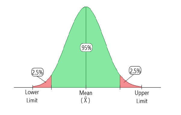
Image Credit: GeeksforGeeks

Formula to calculate Confidence Interval is:

 

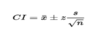
	CI =	confidence interval
	X =	sample mean
	Z =	confidence level value
	S =	sample standard deviation
	N =	sample size

 

Another important term in the confidence interval concept is the margin of error. The margin of error in statistics refers to the degree of error in the results of random sampling surveys. A wider statistical margin of error suggests a reduced likelihood of relying on survey or poll results to accurately reflect a community, implying a lower level of trust in the results.

To conclude, these are the basic understandings of inferential statistics which can be very useful in the studies going forward. We strongly recommend brushing up on the basics of Statistics before jumping into the core of Data Science because the whole foundation of Data Science is built on the strong shoulders of Statistics.

 

---

Author: Vaishnav Mishra (Data Analytics & Business Intelligence Leader)

Author Biography
Vaishnav Mishra is a passionate blogger and Tech content curator.He loves to write on trending topics of “Data Science, Data Analytics & Business Intelligence“He has strong analytical skills, client-facing experience through consulting for multiple stakeholders and active team leadership by managing projects, channelizing efforts, and mentoring peers.

LinkedIn: https://www.linkedin.com/in/vaishnav-mishra-39222b8a

Please below published article on Same Author.

Data Science for Beginners part-1

Data Science for Beginners part-1

Four Easy Steps to Get Subscribed

Step1:-Enter your Email address and Hit SUBSCRIBE Button.

Step2:-Please check inbox and open the email with the subject line“Confirm your subscription for Global PLM“.

Step3:-Please click “Confirm Follow” and you got the email with the subject” Confirmed subscription to posts on Global PLM”.

Step4:-Voila, You are subscribed.Happy Learning

---